hexify

Equal-Area Hexagonal Grids for Global Spatial Analysis

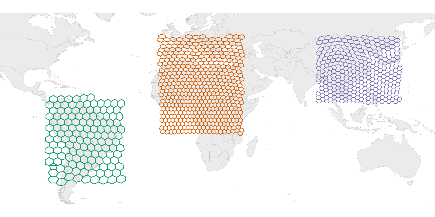
hexify assigns geographic coordinates to equal-area hexagonal grid cells using the ISEA (Icosahedral Snyder Equal Area) projection. Every cell has the same area regardless of latitude, eliminating the sampling bias inherent in rectangular lat-lon grids. H3 is supported for compatibility with existing H3 workflows.

Quick Start

library(hexify)

cities <- data.frame(
  name = c("Vienna", "Paris", "Madrid"),
  lon = c(16.37, 2.35, -3.70),
  lat = c(48.21, 48.86, 40.42)
)

# ISEA equal-area grid (default)
grid <- hex_grid(area_km2 = 10000)
result <- hexify(cities, lon = "lon", lat = "lat", grid = grid)
plot(result)

# H3 grid (Uber's system)
h3_grid <- hex_grid(resolution = 4, type = "h3")
result_h3 <- hexify(cities, lon = "lon", lat = "lat", grid = h3_grid)
plot(result_h3)

Statement of Need

Spatial binning is fundamental to ecological modeling, epidemiology, and geographic analysis. Standard approaches using rectangular lat-lon grids introduce severe area distortions: a 1° cell at the equator covers ~12,300 km², while the same cell near the poles covers a fraction of that area. This violates the equal-sampling assumption underlying most spatial statistics.

Discrete Global Grid Systems (DGGS) solve this by partitioning Earth’s surface into cells of uniform area. hexify’s primary backend is ISEA (Icosahedral Snyder Equal Area): true equal-area hexagonal grids with apertures 3, 4 and 7 in any sequence, implemented in C++ with no external dependencies. For interoperability with industry ecosystems (FCC, Foursquare, DuckDB), hexify also supports H3 grids via a vendored C library.

Equal-area grids are directly applicable to:

• Species distribution modeling and biodiversity assessments
• Epidemiological surveillance and disease mapping
• Environmental monitoring and remote sensing aggregation
• Any analysis requiring unbiased spatial binning

Why Hexagonal Grids?

Hexagons tile the sphere with three properties that squares and triangles lack:

1. Equal area — every cell covers the same surface area, from equator to pole
2. Uniform adjacency — all six neighbors share an edge (no ambiguous diagonal neighbors)
3. Low shape distortion — hexagons approximate circles better than any other regular polygon, minimizing edge effects in spatial statistics

These properties make hexagonal grids the natural choice for unbiased spatial binning. Rectangular lat-lon grids, by contrast, shrink toward the poles: a 1° cell at 60°N has half the area of the same cell at the equator.

Features

Core Workflow

• hex_grid(): Define a grid by target cell area (km²) or resolution level
• hexify(): Assign points to grid cells (data.frame or sf input)
• plot() / hexify_heatmap(): Visualize results with base R or ggplot2
• Any body: hex_grid(area_km2 = 1000, radius_km = "mars") sizes a grid on Mars, the Moon, Titan, or any radius you give — both backends

Grid Generation

• grid_rect(): Generate cell polygons for a bounding box
• grid_global(): Generate a complete global grid (all cells)
• grid_clip(): Clip grid to a polygon boundary (country, region, etc.)

Cell Operations

• cell_to_sf(): Convert cell IDs to sf polygon geometries
• cell_to_lonlat(): Get cell center coordinates
• get_parent() / get_children(): Navigate grid hierarchy

Interoperability

• as_dggrid() / from_dggrid(): Convert to/from dggridR format
• as_sf(): Export HexData to sf object
• as.data.frame(): Extract data with cell assignments
• H3 support: hex_grid(resolution = 8, type = "h3") — vendored H3 C library, no extra install needed

Installation

# Install from CRAN
install.packages("hexify")

# Or install development version from GitHub
# install.packages("pak")
pak::pak("gcol33/hexify")

Usage Examples

Basic Point Assignment

library(hexify)

# Define grid: ~10,000 km² cells
grid <- hex_grid(area_km2 = 10000)
grid
#> HexGridInfo Specification
#> -------------------------
#> Aperture:    3
#> Resolution:  8
#> Area:        7773.97 km^2
#> Diagonal:    94.74 km
#> CRS:         EPSG:4326
#> Total Cells: 65612

# Assign coordinates to cells
coords <- data.frame(
  lon = c(-122.4, 2.35, 139.7),
  lat = c(37.8, 48.9, 35.7)
)
result <- hexify(coords, lon = "lon", lat = "lat", grid = grid)

# Access cell IDs
result@cell_id

Working with sf Objects

library(sf)

# Any CRS works - hexify transforms automatically
points_sf <- st_as_sf(coords, coords = c("lon", "lat"), crs = 4326)
result <- hexify(points_sf, area_km2 = 10000)

# Export back to sf
result_sf <- as_sf(result)

Generating Grid Polygons

# Grid for Europe
grid <- hex_grid(area_km2 = 50000)
europe_hexes <- grid_rect(c(-10, 35, 40, 70), grid)
plot(europe_hexes["cell_id"])

# Clip to a country boundary
library(rnaturalearth)
france <- ne_countries(country = "France", returnclass = "sf")
france_grid <- grid_clip(france, grid)

Aggregating Point Data

# Species occurrence data
occurrences <- data.frame(
  species = sample(c("Sp A", "Sp B", "Sp C"), 1000, replace = TRUE),
  lon = runif(1000, -10, 30),
  lat = runif(1000, 35, 60)
)

# Assign to grid
grid <- hex_grid(area_km2 = 20000)
occ_hex <- hexify(occurrences, lon = "lon", lat = "lat", grid = grid)

# Count per cell
occ_df <- as.data.frame(occ_hex)
occ_df$cell_id <- occ_hex@cell_id

cell_counts <- aggregate(species ~ cell_id, data = occ_df, FUN = length)
names(cell_counts)[2] <- "n_records"

# Richness per cell
richness <- aggregate(species ~ cell_id, data = occ_df,
                      FUN = function(x) length(unique(x)))
names(richness)[2] <- "n_species"

Visualization

# Quick plot
plot(result)

# Heatmap with basemap
hexify_heatmap(occ_hex, value = "n_records", basemap = TRUE)

# Custom ggplot
library(ggplot2)
cell_polys <- cell_to_sf(cell_counts$cell_id, grid)
cell_polys <- merge(cell_polys, cell_counts, by = "cell_id")

ggplot(cell_polys) +
  geom_sf(aes(fill = n_records), color = "white", linewidth = 0.2) +
  scale_fill_viridis_c() +
  theme_minimal()

Known Limitations

• H3 grids: Fixed aperture 7, maximum resolution 15 (~0.9 m² cells). ISEA grids support apertures 3, 4 and 7 in any sequence up to resolution 30.
• Pentagons: Any hexagonal tiling of a sphere requires exactly 12 pentagonal cells (at icosahedron vertices). These cells have 5 neighbors instead of 6. Use is_pentagon() to detect them.
• Projection precision: The inverse Snyder projection uses iterative Newton-Raphson convergence. Default precision is sufficient for sub-meter accuracy; use hexify_set_precision() to adjust the speed/accuracy trade-off.

Documentation

• Quick Start - Basic concepts and workflow
• Visualization - Plotting with base R and ggplot2
• Workflows - Grid generation, clipping, multi-resolution analysis

Support

“Software is like sex: it’s better when it’s free.” — Linus Torvalds

I’m a PhD student who builds R packages in my free time because I believe good tools should be free and open. I started these projects for my own work and figured others might find them useful too.

If this package saved you some time, buying me a coffee is a nice way to say thanks. It helps with my coffee addiction.

Citation

@software{hexify,
  author = {Colling, Gilles},
  title = {hexify: Equal-Area Hexagonal Grids for Spatial Analysis},
  year = {2025},
  url = {https://CRAN.R-project.org/package=hexify},
  doi = {10.32614/CRAN.package.hexify}
}

License

MIT (see LICENSE.md)